Image Processing

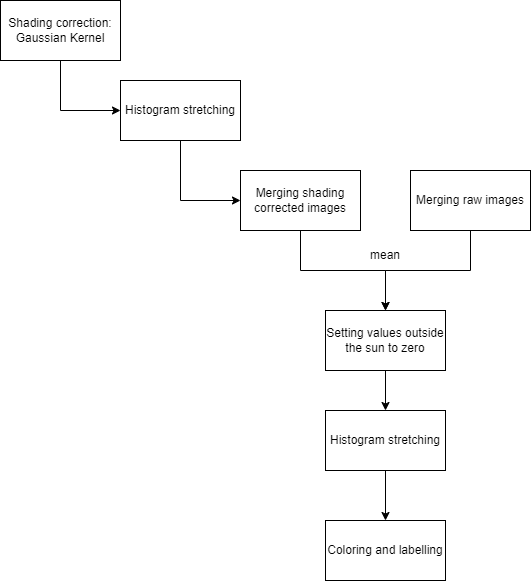
This script is for image processing. It takes pictures of the sun with different exposure times edits them and merges them together afterwards. In the end it colors the final image and labels it with time and location of the image taken.

Code Description

In this part of the documentation the code is split up in different sections of the image processing.

Shading Correction

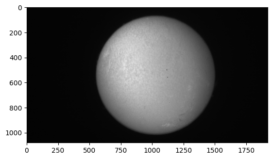
The shading correction is needed because the telescope produces a shading on the images that are made with a CMOS camera. Like you can see here:

The Gaussian Kernel is set to a big size and a high sigma. It is applied in the spatial domain. With this Kernel the image gets blurred so far that we only the shadows produced by the telescope remain. In astronomy this is often reffered to as flat field correction. The Kernel is applied with the filter2d function from cv2.

gaussian_kernel = cv2.getGaussianKernel(kernel_size, sigma)
gaus = cv2.filter2D(img, cv2.CV_8U, kernel=gaussian_kernel_2d)

The parameters have the following meaning:

• kernel_size: Choosing the size of the Kernel. For example 256 so that the kernel is big enough and only the pattern of the shadow remains.

• sigma: Sigma is the Gaussian standart deviation

Afterwards the original image is divided by its shadow pattern to get a shadow corrected image.

Histogramm stretching

To obtain the complete dynamic range from 0 to 255 the histogramm is stretched with the following formula:

\[ \frac{{(\text{sharpened} - \text{min_value}) \cdot (\text{new_max} - \text{new_min})}}{{\text{max_value} - \text{min_value}} + \text{new_min}} \]

The parameters are determined as follows:

• sharpened: The image which you wanna stretch over the whole dynamic range.

• min_value and max_value: This are values which determine the range of the histogramm with values that are important for the stretching of the histogramm.

• new_min and new_max: This values represent the new range of the histogramm: mostly they are set to 0 and 255.

This function is used several times to not loose any structure while processing the image. For example after cutting out the sun the histogram stretching is applied to highlight the structure of the border and the inside of the sun.

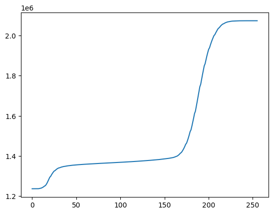
Getting the peaks of the histogramm

To get the sections with important structures you try to extract the parts of the histogram where it has a peak. This is done with analysing the CDF function of the histogram. The parts where the CDF function doesn't change more than a certain value are extracted and used to determine min_valueand max_value for the histogram stretching.

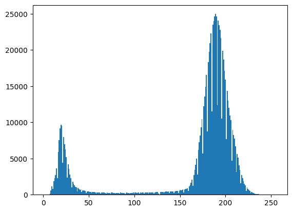
The peak on the left marks the structure on the border and the peak on the right the structure on the inside. To extract the min_value and max_value for later stretching the cdf function is used:

Merging the images

To merge the images with different exposure times the Algorithm from Mertens is used. To process the images With the function MergeMertens.process from cv2 you have to give the function a list with differently exposed images.

compensator = cv2.createMergeMertens()
data_image = compensator.process(gaus_images)

Firstly the raw images gets stacked and secondly the images with the shadow correction are stacked. Afterwards the mean of this two images is taken to ensure that the values of the image are not to high nor to low.

Cutting out the sun

To make sure that everything outside the sun is set to 0 the center is calculated with the HoughCircles function from cv2.

Afterwards you determine the radius where the sun ends with the function plot_values_for_radii. This is then used to set every value outside the sun to 0.

Coloring the Image

To color the image in Halpha the command LinearSegmentedColormap from Matplotlib with which you can make a personalised Colormap is used.

cmap = LinearSegmentedColormap.from_list('halpha_cmap', ['black', 'red'], N=256)

In this case it is made from black to red because the images that are taken of the sun are in Halpha wavelenght.

Labeling the image

To give the images a more scientific look they get labeled with the positions of the poles, the location of the observatory and the time when the image was taken. The image gets labeled with the write_text function which uses the putText function from cv2.

Usage

This image processing script is mainly used in our application for the livestream. It follows the alignment of the raw images. The whole script for the livetstream can be found here.

Sources

The idea of the shadow correction with a Gaussian Kernel and the following Division is taken from pages 173 and 174 of: - Rafael C. Gonzalez, Richard E. Woods 2018, Digitale Image Processing Fourth edition, Pearson.

The functions where mainly build with OpenCV, NumPy, Matplotlib.

Python Script

The python script can be found here.